GOOGLESHEET Function
This article explains how to use GOOGLESHEET functions
Live
Fast-track your calculator
30-min onboarding session with + Live Q&A
FSGOOGLESHEET("1qYJVonS_caYCc1diSOYb0HM-s5nUyxW6PsfsvzIoJK9I", "2050638375")
Syntax
FSGOOGLESHEET(spreadsheet_id, sheet_id)
spreadsheet_id- The IDstringof the Google spreadsheet that can be found in the URL of the spreadsheetsheet_id- The IDstringof the sheet (or sometimes called worksheet) that can be found in the URL of the spreadsheet.
Notes
- Before you can use the GOOGLESHEET function you need to connect your Google account. You can connect your account in the connections section of the account page.
- The return value from this function is a matrix (or table-like dataset) with rows and columns.
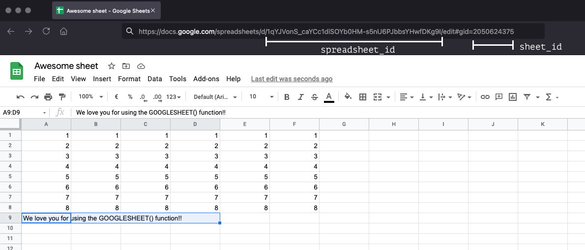
- You can find the
spreadsheet_idandsheet_idin the URL of your Google spreadsheet. Open your spreadsheet and find thespreadsheet_idandsheet_idhere:
Examples
You can use the data from the GOOGLESHEET function exactly as you would use data from datasheets. Here are some examples:
Returning a single value from the matrix
If you want to return a single value, you can do so in conjunction with the INDEX function:
FSINDEX(GOOGLESHEET("spreadsheet_id", "sheet_id"), 0, 0)
FSINDEX(GOOGLESHEET("spreadsheet_id", "sheet_id"), QA, QB)
FSVLOOKUP(123, GOOGLESHEET("spreadsheet_id", "sheet_id"), 1, 0)
FSVLOOKUP(QA{text}, GOOGLESHEET("spreadsheet_id", "sheet_id"), QB, 1)
Now we're talking! If a user fills out a text field, it searches all the rows of the first column of your spreadsheet to find a partial match. Depending on the value of QB it returns that column.
Using SUMIF, SUMIFS, FINDIF, FINDIFS
Using SUMIF, SUMIFS, and FINDIFS is possible as well. It works a little bit differently when using GOOGLESHEET() compared to datasheets:
Datasheet
FSSUMIFS(DA_C, DA_A, QA, DA_B, QB)
GOOGLESHEET()
FSVA = GOOGLESHEET("spreadsheet_id", "sheet_id")

FINDIFS(COLUMN(VA, 2), COLUMN(VA, 0), QA, COLUMN(VA, 1), QB)
In this example we first created a variable (VA) for getting the spreadsheet data. then for FINDIFS we need to reference the columns A, B, and C a little bit differently:
- DA_C = COLUMN(VA, 2)
- DA_A = COLUMN(VA, 0)
- DA_B = COLUMN(VA, 1)
Note that counting starts at 0, so the first column (A) is referred to as 0, the second column as 1, etc.
This works the same for SUMIF and SUMIFS.
Troubleshoot issues
- If your GoogleSheet contains merged cells, the formula will throw a
#NAME-error. This error occurs when the app doesn't recognize something in your formula. In this case, the merged fields provide an unexpected input. - Some browsers like Opera have aggressive caching mechanisms that prevent your GoogleSheet data from updating in real-time. When you run into this problem, try switching to an alternative browser like Chrome or Safari.